mètodos de ordenamento, PCA e NMDS
Felipe Melo
2022-01-31
Análise de Componentes Principais
Slides
Exercícos para PCA e NMDS
Imagine que você precisa entender commo se agrupam as comunidades do rio que estamos estudando. Essa necessidade vem do fato de que um usina hidroelétrica está para ser construída no rio e o governo encomendou estudos de impacto ambiental que precisam demonstrar várias coisas. Você como biólogo, que está preocupado com o rio, precisa converncer o governo de construir a hidroelétrica num stor do rio que tenha o menor impacto possível. Para isso, você vai precisar anaalisar tanto a comunidade de peixes quanto as condições fisico-químicas do rio.
Passo 1 - Faça uma PCA pra a tabela “env” (excluindo as colunas ‘dfs’ e ‘dis’). Seu intuito em vez de dividir o rio de maneira arbitrária é encontrar divisões naturais de características ambientais, que possam ser separadas pelo seu valor médio. Examine os PCs 1 e 2 e veja, através de historgramas em quantas porçoes o rio pode ser dividido.
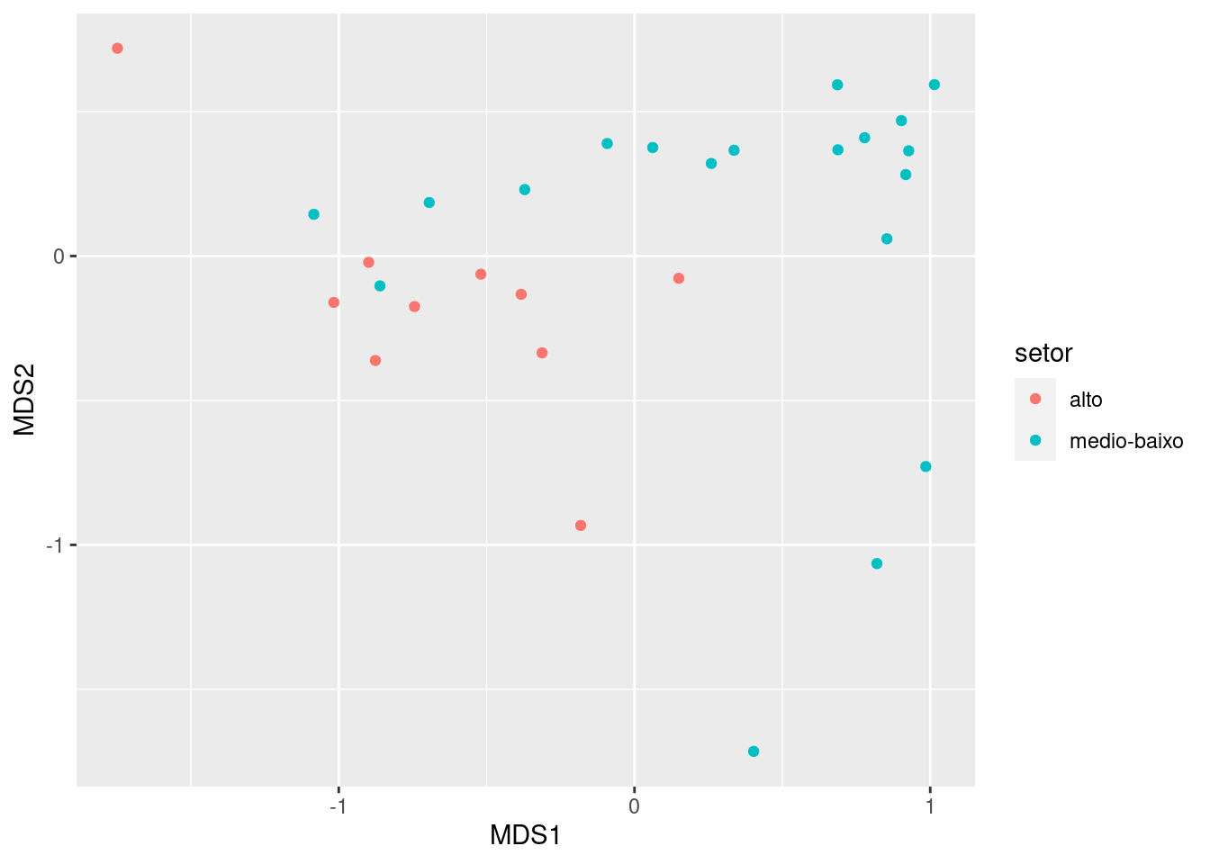
Passo 2 - Faça um NMDS para os dados da comunidade biológica “spe” e use as mesmas categorias que você encontrou no passo anterior para pintas as amostras. Será que há uma coincidência?
Passo 3 - Use o métodos de K-means para gerar agrupamentos automáticos e veja se eles coincidem com os que você gerou usando o método anterior
veja este exemplo simplificado
env_simp<-env[,2:4] # escolhi apenas três variáveis
princomp(env_simp)-> pca_env
summary(pca_env)
## Importance of components:
## Comp.1 Comp.2 Comp.3
## Standard deviation 267.2654510 8.881811549 7.5185567870
## Proportion of Variance 0.9981078 0.001102288 0.0007898794
## Cumulative Proportion 0.9981078 0.999210121 1.0000000000Analisei os PCs e vi que o PC1 (Comp.1) concentra quase toda informação
library(tidyverse)
pca_env$scores %>%
  as.tibble() %>%
  ggplot(aes(Comp.1))+geom_histogram()
## Warning: `as.tibble()` was deprecated in tibble 2.0.0.
## Please use `as_tibble()` instead.
## The signature and semantics have changed, see `?as_tibble`.
## This warning is displayed once every 8 hours.
## Call `lifecycle::last_lifecycle_warnings()` to see where this warning was generated.## `stat_bin()` using `bins = 30`. Pick better value with `binwidth`.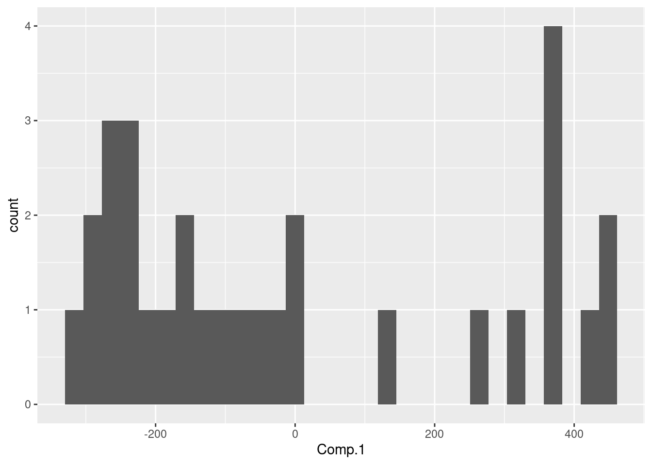
Então, decidi dividr rio em duas porções uma com valores negativos do PC-1 e outr com os valores positiovs desse memso PC. Daí uso os valores do vetor do PC-1 para criar minha categoria de “setores do rio”.
pca_env$scores %>%
as.tibble() %>%
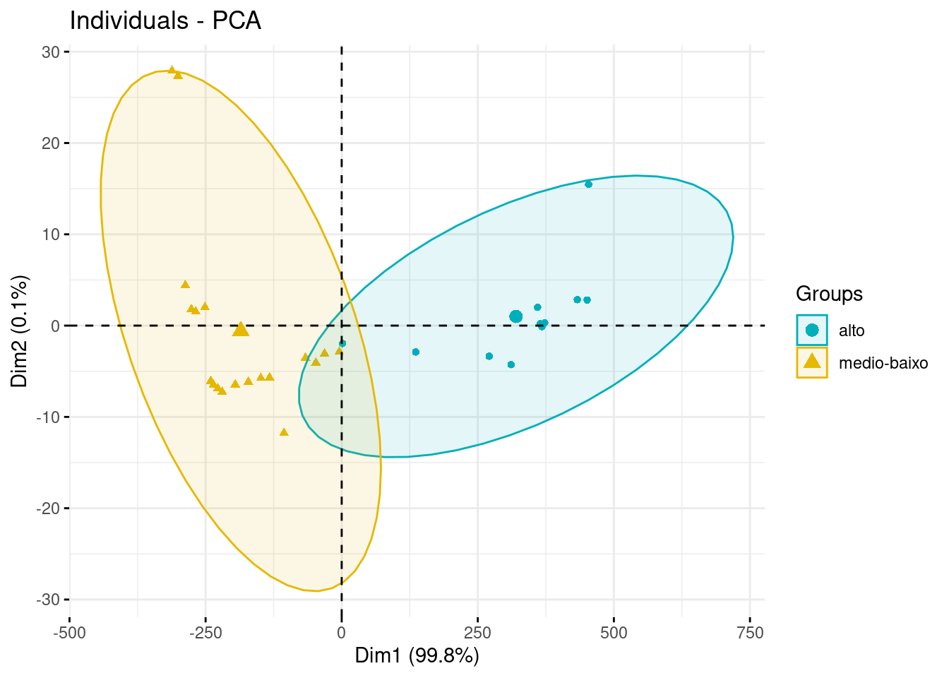
mutate(setor=ifelse(Comp.1<0,"medio-baixo", "alto"))-> env_set
library(factoextra)
fviz_pca_ind(pca_env,
geom.ind = "point", # show points only (nbut not "text")
col.ind = env_set$setor, # color by groups
palette = c("#00AFBB", "#E7B800"),
addEllipses = TRUE, # Concentration ellipses
legend.title = "Groups"
)
Agora o NMDS
nmds<-metaMDS(spe[-8,-c(20:30)]) # exclui algumas espécies spo para não dar de bandeja## Run 0 stress 0.08903472
## Run 1 stress 0.1295109
## Run 2 stress 0.1114362
## Run 3 stress 0.08903464
## ... New best solution
## ... Procrustes: rmse 0.0002047508 max resid 0.000981429
## ... Similar to previous best
## Run 4 stress 0.1206846
## Run 5 stress 0.1321453
## Run 6 stress 0.1174552
## Run 7 stress 0.0917874
## Run 8 stress 0.08903478
## ... Procrustes: rmse 0.0001682073 max resid 0.0008076618
## ... Similar to previous best
## Run 9 stress 0.1286358
## Run 10 stress 0.115941
## Run 11 stress 0.1294656
## Run 12 stress 0.1152777
## Run 13 stress 0.1180302
## Run 14 stress 0.09178715
## Run 15 stress 0.1305705
## Run 16 stress 0.1156196
## Run 17 stress 0.1333929
## Run 18 stress 0.1334706
## Run 19 stress 0.09178721
## Run 20 stress 0.1165492
## *** Solution reachednmds$points## MDS1 MDS2
## 1 -1.7483712 0.71926728
## 2 -1.0165858 -0.16047209
## 3 -0.8987585 -0.02173984
## 4 -0.5193284 -0.06279278
## 5 0.1498353 -0.07708280
## 6 -0.3832489 -0.13239063
## 7 -0.7437180 -0.17484421
## 9 -0.1817967 -0.93271913
## 10 -0.3123741 -0.33518763
## 11 -0.8759671 -0.36165802
## 12 -0.8607013 -0.10326571
## 13 -1.0843178 0.14448101
## 14 -0.6940532 0.18540318
## 15 -0.3711233 0.23015167
## 16 -0.0921675 0.38962692
## 17 0.0616789 0.37573115
## 18 0.2597215 0.32049460
## 19 0.3365941 0.36623218
## 20 0.6878717 0.36801807
## 21 0.7781309 0.40959751
## 22 0.9026005 0.46884237
## 23 0.4028798 -1.71494524
## 24 0.8196447 -1.06469202
## 25 0.9850631 -0.72870248
## 26 0.8535780 0.05978260
## 27 0.9173160 0.28208132
## 28 0.9271782 0.36440451
## 29 0.6863051 0.59287056
## 30 1.0141139 0.59350765
## attr(,"centre")
## [1] TRUE
## attr(,"pc")
## [1] TRUE
## attr(,"halfchange")
## [1] TRUE
## attr(,"internalscaling")
## [1] 1.065256nmds_dat<-data.frame(nmds$points, env_set$setor[-8])
colnames(nmds_dat) <- c("MDS1","MDS2","setor")Vamos ao gráfico do NMDS
nmds_dat %>%
  ggplot(aes(MDS1, MDS2, color=setor))+geom_point()