class: center, middle, inverse, title-slide # Ecologia Numérica ## Métodos de ordenamento ### Felipe Melo ### Laboratório de Ecologia Aplicada - UFPE ### 2022-01-31 --- # Análise de Componentes Principais - PCA .center[ 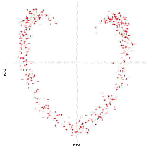<!-- --> ### fonte: [David Zelený](https://www.davidzeleny.net/anadat-r/doku.php/en:start) ] --- .pull-left[ # O que precisamos saber? ###- Uma PCA é um método limdear de agrupamento ###- Está baseada no princípio dos *"duplos zeros"* ###- É um método para reduzir a multi-dimensionalidade dos dados ###- Tem um mooooonte de tutorial por aí... ] .pull-right[ <img src="https://miro.medium.com/max/2112/1*_NK2wo5o0ngQ-MfdoXe1aw.png" height=500> ] --- # O princípio é simples... SQN .center[ <img src="https://www.davidzeleny.net/anadat-r/lib/exe/fetch.php/obrazky:pca_algorithm_2d_legendre-legendre.jpg?cache=&w=639&h=473&tok=d5cead">] --- <iframe width="1195" height="672" src="https://www.youtube.com/embed/HMOI_lkzW08" title="YouTube video player" frameborder="0" allow="accelerometer; autoplay; clipboard-write; encrypted-media; gyroscope; picture-in-picture" allowfullscreen></iframe> --- # Entendeu? Não? .panelset[ .panel[.panel-name[Base] ```r head(iris) # Dados sobre três espécies de planta que diferem em algumas características ``` ``` ## Sepal.Length Sepal.Width Petal.Length Petal.Width Species ## 1 5.1 3.5 1.4 0.2 setosa ## 2 4.9 3.0 1.4 0.2 setosa ## 3 4.7 3.2 1.3 0.2 setosa ## 4 4.6 3.1 1.5 0.2 setosa ## 5 5.0 3.6 1.4 0.2 setosa ## 6 5.4 3.9 1.7 0.4 setosa ``` ] .panel[.panel-name[PCA] ```r iris.pca <- PCA(iris[,-5], graph = FALSE) iris.pca ``` ``` ## **Results for the Principal Component Analysis (PCA)** ## The analysis was performed on 150 individuals, described by 4 variables ## *The results are available in the following objects: ## ## name description ## 1 "$eig" "eigenvalues" ## 2 "$var" "results for the variables" ## 3 "$var$coord" "coord. for the variables" ## 4 "$var$cor" "correlations variables - dimensions" ## 5 "$var$cos2" "cos2 for the variables" ## 6 "$var$contrib" "contributions of the variables" ## 7 "$ind" "results for the individuals" ## 8 "$ind$coord" "coord. for the individuals" ## 9 "$ind$cos2" "cos2 for the individuals" ## 10 "$ind$contrib" "contributions of the individuals" ## 11 "$call" "summary statistics" ## 12 "$call$centre" "mean of the variables" ## 13 "$call$ecart.type" "standard error of the variables" ## 14 "$call$row.w" "weights for the individuals" ## 15 "$call$col.w" "weights for the variables" ``` ] .panel[.panel-name[Gráfico] <!-- --> ] .panel[.panel-name[Gráfico2] <!-- --> ] ] --- # Como interpretamos? .panelset[ .panel[.panel-name[ex-1] <img src="slides_aula4_ordenacao_files/figure-html/unnamed-chunk-7-1.png" width="400px" /> ] .panel[.panel-name[ex-2] <img src="slides_aula4_ordenacao_files/figure-html/unnamed-chunk-8-1.png" width="400px" /> ] .panel[.panel-name[ex-3] <img src="slides_aula4_ordenacao_files/figure-html/unnamed-chunk-9-1.png" width="400px" /> ] .panel[.panel-name[ex-4] <img src="slides_aula4_ordenacao_files/figure-html/unnamed-chunk-10-1.png" width="400px" /> ] ] --- # Autovetores (eigenvalues) .panelset[ .panel[.panel-name[objetos 'PCA'] ```r iris.pca ``` ``` ## **Results for the Principal Component Analysis (PCA)** ## The analysis was performed on 150 individuals, described by 4 variables ## *The results are available in the following objects: ## ## name description ## 1 "$eig" "eigenvalues" ## 2 "$var" "results for the variables" ## 3 "$var$coord" "coord. for the variables" ## 4 "$var$cor" "correlations variables - dimensions" ## 5 "$var$cos2" "cos2 for the variables" ## 6 "$var$contrib" "contributions of the variables" ## 7 "$ind" "results for the individuals" ## 8 "$ind$coord" "coord. for the individuals" ## 9 "$ind$cos2" "cos2 for the individuals" ## 10 "$ind$contrib" "contributions of the individuals" ## 11 "$call" "summary statistics" ## 12 "$call$centre" "mean of the variables" ## 13 "$call$ecart.type" "standard error of the variables" ## 14 "$call$row.w" "weights for the individuals" ## 15 "$call$col.w" "weights for the variables" ``` ] .panel[.panel-name[objetos prcomp] ```r iris.prcomp<-prcomp(iris[,-5], scale. = TRUE) iris.prcomp ``` ``` ## Standard deviations (1, .., p=4): ## [1] 1.7083611 0.9560494 0.3830886 0.1439265 ## ## Rotation (n x k) = (4 x 4): ## PC1 PC2 PC3 PC4 ## Sepal.Length 0.5210659 -0.37741762 0.7195664 0.2612863 ## Sepal.Width -0.2693474 -0.92329566 -0.2443818 -0.1235096 ## Petal.Length 0.5804131 -0.02449161 -0.1421264 -0.8014492 ## Petal.Width 0.5648565 -0.06694199 -0.6342727 0.5235971 ``` ] .panel[.panel-name[autovetores PCA] ```r iris.pca$eig ``` ``` ## eigenvalue percentage of variance cumulative percentage of variance ## comp 1 2.91849782 72.9624454 72.96245 ## comp 2 0.91403047 22.8507618 95.81321 ## comp 3 0.14675688 3.6689219 99.48213 ## comp 4 0.02071484 0.5178709 100.00000 ``` ] .panel[.panel-name[autovetores prcomp] ```r summary(iris.prcomp) ``` ``` ## Importance of components: ## PC1 PC2 PC3 PC4 ## Standard deviation 1.7084 0.9560 0.38309 0.14393 ## Proportion of Variance 0.7296 0.2285 0.03669 0.00518 ## Cumulative Proportion 0.7296 0.9581 0.99482 1.00000 ``` ]] --- # Resumo dos autovetores .pull-left[ <img src="https://upload.wikimedia.org/wikipedia/commons/0/06/Eigenvectors.gif"> ] .pull-right[ <img src="https://wiki.pathmind.com/images/wiki/mona_lisa_eigenvector.png"> ] credit: [Chris Nicholson](https://wiki.pathmind.com/eigenvector) --- # Resumo dos autovetores .pull-left[ ###- São o valor que informa quanta relação há entre variáveis ###- Informam a direção da vairação [Aqui tem ums explicação maravilhosa](https://setosa.io/ev/principal-component-analysis/)] .pull-right[ <img src="https://i.stack.imgur.com/lNHqt.gif" > ] --- # Quantos PCs devo usar para entender meu fenômeno? .center[ ```r fviz_eig(iris.prcomp) ``` 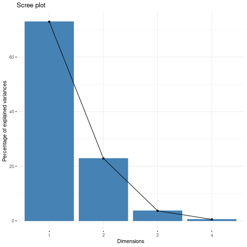<!-- --> ] --- # Qualidade da representação .center[ ``` ## Warning: ggrepel: 19 unlabeled data points (too many overlaps). Consider ## increasing max.overlaps ``` 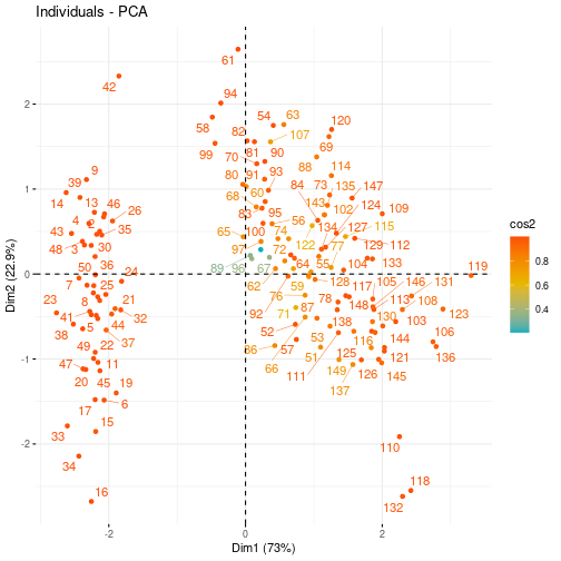<!-- --> ] --- # Qualidade da representação .center[ 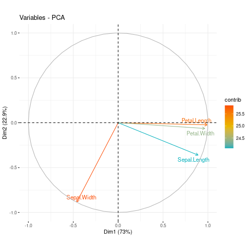<!-- --> ] --- class: center, middle # Dúvidas